2. How to create the lease amortization schedule and calculate your lease liability
- Create five-column spreadsheet
- Enter the number of periods and cash payments
- Enter expense formula
- Fill expense column
- Enter liability reduction formula
- Enter liability balance formula
- Fill remaining liability balance
- Perform “What-If Analysis” on liability balance
- Set liability balance value to 0 with goal seek
- Click “OK”
Private companies in particular may be tempted to try to use an Excel spreadsheet for lease accounting, but this information is important even if you plan to use lease accounting software for compliance with the new standard. You can use the information in this blog to ensure that your chosen software provider is performing this calculation accurately. Transitioning to ASC 842, IFRS 16, and GASB 87 can be difficult, but there are resources that can help you gain an understanding of the methods laid out below for our calculations.

What is the lease liability?
The lease liability is defined as the present value of your future lease payments. This is calculated as the initial step in accounting for a lease under ASC 842, and this amount is then used to calculate the ROU (right-of-use) asset, that is recorded in addition to the liability for operating leases and capital leases.
A lessee’s obligation to make the lease payments arising from a lease, measured on a discounted basis.
How to create the lease amortization schedule and calculate your lease liability
Download our free present value calculator to follow along:

Follow the steps below to calculate the present value of lease payments and the lease liability amortization schedule using Excel when the payment amounts are not constant, illustrated with an example:
Calculate the present value of lease payments for a 10-year lease with annual payments of $1,000 with 5% escalations annually, paid in advance. Assume the rate inherent in the lease is 6%.


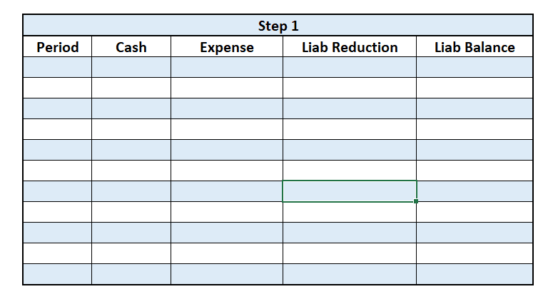
Step 1: Create an Excel spreadsheet with these five columns
Create a new Excel spreadsheet and title five columns with the following headers: Period, Cash, Expense, Liability Reduction, and Liability Balance, as shown below:
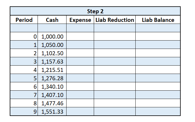
Step 2: Enter the number of periods and cash payments
Enter the number of periods corresponding to the lease term starting from 0, and enter the cash payments in each period. Because payments are made in advance, the first payment of $1,000 is made in period 0. The annual payments then escalate at a 5% rate. Please see illustration below:
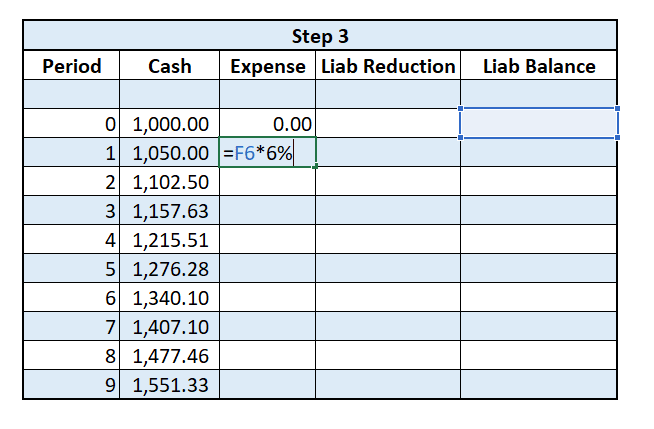
Step 3: Enter the expense formula
Enter “0” for expense in period 0 (because payments are made in advance). In Expense for period 1, enter the cell reference for the period 0 liability balance and multiply by 6%. See below.
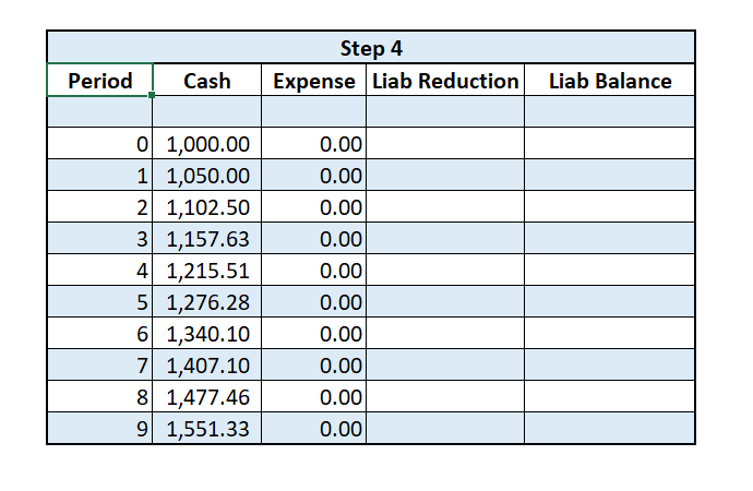
Step 4: Fill the expense column
Copy the formula for expense in period 1 down for the remaining Expense rows.
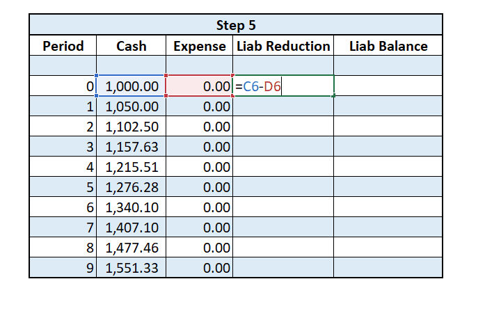
Step 5: Enter the formula for liability reduction
The formula for each liability reduction amount is the corresponding cash payment minus the corresponding expense. See below.
 Copy the formula down the entire Liability Reduction column.
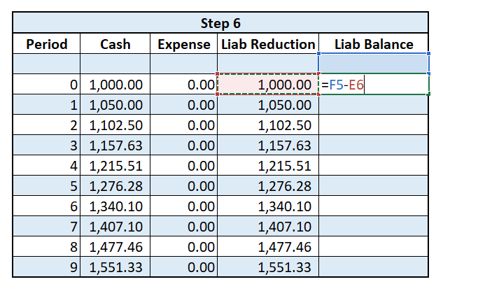
Step 6: Enter the formula for liability balance
Enter “0” for the Liability Balance in the line above period 0. In liability balance for period 0, enter the formula for the above cell’s liability balance minus the liability reduction in period 0. This will equal the previous period’s liability balance, reduced by the current liability reduction (see below).
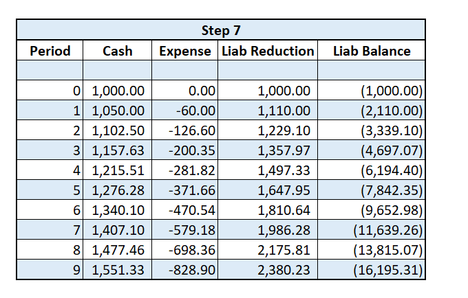
Step 7: Fill the remaining liability balance column
Copy the formula for the liability balance in period 0 down for the remaining Liability Balance rows.
Step 8: Perform “What-If Analysis” on the liability balance
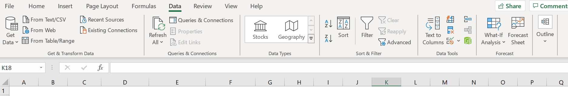
Select the liability balance for period 9. In the top bar in Excel, go to the “Data” tab, then the “What-if Analysis” Tab, then select “Goal Seek.”
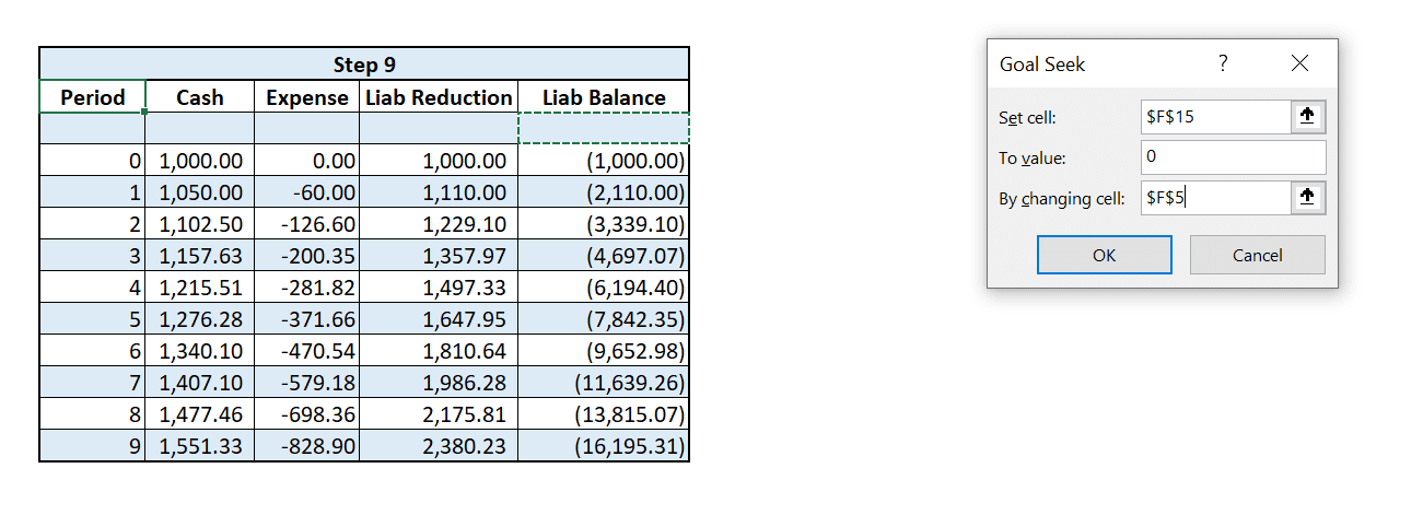
Step 9: Set liability balance value to 0 by using goal seek
In the dialog box that follows, make sure “Set cell” is set to the cell representing the liability balance for period 9, in the “To Value” enter 0, and in “By changing cell” enter the cell reference representing the liability balance for the period above period 0. See below.
Step 10: Click “OK”
Click “OK” to have Excel run the goal seek analysis. Excel will provide the beginning liability balance and your amortization schedule will be completed automatically as a result of the formulas you input. See below.
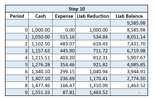
For this example, the present value of a 10-year lease with payments of $1,000 annually, 5% escalations, and a rate inherent in the lease of 6% is $9,586.
Summary
This schedule will provide you with the calculations for your journal entries for the entire life of the lease, if you’re using Excel. If you’re using a lease accounting software, the information above will help you cross-check the calculations performed by your provider so you can ensure accuracy.